Take it from a true bonehead (just ask my wife or kids…)

As I mentioned in an earlier post, I’ve spent some time thinking about the relationship between low density lipoprotien (LDL)–or bad cholesterol–and CV events.  Now that I’ve got a few minutes to spare and the kids are in bed, it’s about time I organize those thoughts and pen a second post (in a three–or maybe four–post series) about them.

In my previous post, I extracted some data from previously published studies and recreated, what I consider to be, one of the most prolific meta-visualizations of trial evidence in cardiovascular disease. To be perfectly honest, my reasons for doing so were not just to have fun with R (I know–it’s a sickness), but to explore the underlying functional form of the model itself. To be specific, the TNT authors and at least one other analyses of similar data appear to all make the same assumption with respect to the linearity of the relationship between LDL and CV events (i.e., not only is lower better, but lower is better at a constant rate). In my review of the literature–which I will admit, may not be the most extensive–I could find only one report from the Cleveland Clinic Journal of Medicine which clearly suggested a nonlinear relationship between LDL and CV events (albeit across a mixture of primary and secondary prevention studies).

Practically speaking, the assumption of linearity may not result in any issues so long as readers confine their interpretations to a “reasonable” range of LDL levels, and practice caution not to extrapolate beyond the range of evaluated LDL values; however, newer–yet to be marketed–cholesterol lowering agents may make it possible for clinicians to take patient LDL levels to lows not readily achieved with any existing medications. In trying to assess the value of these new cholesterol lowering medications (provided they make it to approval), reimbursement agencies and health technology assessment organizations will have to rely on modeling to evaluate the long term clinical benefits. As a health outcomes researcher, I am acutely aware of how assumptions like the one I mention above can substantially alter the outcome of any modeling exercises. Especially in cases that depend on extraplating beyond the bounds of which you have data, ensuring you have the right model is extremely important.  For this reason, it is vial that we re-consider the implied assumption of linearity and at the very least apply sensitivity analyses when modeling any outcomes dependent upon the relationship of LDL  and CV events.

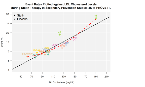
Since my previous post, I’ve extracted data from a few more secondary prevention trials (PROVE-IT and IDEAL). For the most part, the outcomes extracted include only those that captured CV death or non-fatal MI. You may notice that I did not include AtoZ. This was an intentional omission as the composite end point in this trial included hospital readmission for ACS.

First, take a look at the bivariate plot of LDL to CV events. Through this plot, you will notice that I have drawn both the OLS regression line (black solid) AND the quadratic regression line (red hashed).

options(stringsAsFactors)
library(RColorBrewer)
file <- "http://dl.dropboxusercontent.com/u/27644144/secprevstatin.csv"
statins <- read.csv(file, header=T) # read raw data from dropbox
statins <- statins[ which(statins$Study != “AtoZ”),] # remove AtoZ
statins$year <- as.numeric(substr(statins$lastrand, 1, 4)) + round(as.numeric(substr(statins$lastrand, 5, 6))/13, 2) # code year -- to be used later as feature

df1 <- statins
yval <- 'eventrate'
pyval <- 'Event (%)'
xval <- 'LDL'
pxval <- 'LDL Cholesterol (mg/dL)'
par(mar=c(5.1, 4.1, 4.1, 12))
df1$pchvec <- ifelse( grepl(“PBO”, df1$Cohort), 1, 19 )
plot( df1[, xval], df1[, yval], type=“n”, ylim=c(0,30), xlim=c(40,210), yaxt='n', xaxt='n', ylab=““, xlab=““)
u <- par(“usr”)
rect(u[1], u[3], u[2], u[4], col = “grey95”, border = “black”)
par(new=T)
abline(h = c(0, 5, 10, 15, 20, 25, 30), col='white', lwd=2) ##  draw h lines
abline(v = c(50,70, 90, 110, 130, 150, 170, 190, 210), col='white', lwd=2) ##  draw v lines
par(new=T)
plot( df1[, xval], df1[, yval], pch=df1$pchvec, col= cpal , bg= df1$pchfill, cex=1.5  ,yaxt='n', xaxt='n', ylab=““, xlab=““, ylim=c(0,30), xlim=c(40,210), lwd=2)
axis(side=2, at=c(0, 5, 10, 15, 20, 25, 30), labels=c(“0”,”5”,'10', '15', '20', '25', '30'), las=1 )
axis(side=1, at=c(50, 70, 90, 110, 130, 150, 170, 190, 210), labels=c(“50” , “70”, “90”, “110”, “130”, “150”, “170”, “190”, “210”)  )
legend( “topleft”, pch=c(19, 1), legend=c(“Statin”, “Placebo”), cex=1.2, border= “n”, bty='n')
text(df1[, xval], df1[, yval], labels = df1$Study, pos = 3, font=2, col=cpal)
title(main=“Event Rates Plotted against LDL Cholesterol Levels\nduring Statin Therapy in Secondary-Prevention Studies 4S to PROVE-IT.”, ylab=pyval, xlab=pxval)
abline(lm(df1$eventrate~df1$LDL), lwd=2)
poly.plot <- lm(eventrate~poly(LDL, 2), data=df1)
poly.pred <- predict(poly.plot, df1[xval])
preddf <- data.frame(x = df1[,xval], y=poly.pred)
preddf <- preddf[ order(preddf$x),]
lines(x=preddf$x, y=preddf$y, type=“l”, col=“red”, lwd=3, lty=2)

From 4S to PROVE-IT

Next, let’s estimate the RMSE for the linear and quadratic functions.

lmmod <- lm(eventrate~LDL, data=statins)
poly <- lm(eventrate~poly(LDL, 2), data=statins)

lmpred <- predict(lmmod, statins)
lmquad <- predict(poly, statins)

rmse.linear <- sqrt(mean((statins$eventrate-lmpred)^2))
rmse.quad <- sqrt(mean((statins$eventrate-lmquad )^2))
rmse.linear
#[1] 2.339196
rmse.quad
#[1] 1.994463

While I walked through the steps, it should come as no surprise that the model with more parameters did a better job fitting the data. The question now is: did the quadratic model overfit the data? Some additional interesting questions might be to consider how valid it might be to include some of the older studies (e.g., 4S) in an analysis like this? When the 4S trial was conducted, many advances in the pharmacologic treatment of high blood pressure and other risk factors known to reduce the risk of a second heart attack were yet to become part of common clinical practice (e.g., post-MI discharge order sets including BB, ACE/ARB, and antiplatelet therapy). Is there a way to use statistics to support removing 4S from our analysis? To take a stab at answering those questions and more, I will walk through some additional analyses in my next 2 or so posts.