
I’ve been playing around with using R for simulations recently, and I ran into a use case that required I sample from a skewed distribution with min and max values of 0 and 1. A beta distribution was a nice representative form (http://en.wikipedia.org/wiki/Beta_distribution#Mode), and base R has a built in rbeta function; however, I needed to be able to feed into rbeta the proper alpha and beta parameters to produce the required distribution. So, I created two simple R functions that allowed me to start with an alpha value (take your pick) and either a target mean or mode, and the function produced the appropriate beta that I could then use to produce a beta distribution and my random sample.
# first by mean
a1 <- 20
mu1 <- .95
solmean <- function(alpha, mean) (alpha-(mean*alpha))/mean
beta <- solmean(a1, mu1)
x1 <- (rbeta(1000, shape1=a1, shape2=beta)) # sample of n=1000 from the beta dist
head(x1)
x1 <- round(x1,3)
hist(x1, breaks=100)# let's give it a look
mean(x1)
x2 <- table(x1)
which.max(x2) # let's see what the mode is
quantile(x1) # more descriptives
# Now by mode
a2 <- 20
mo1 <- .95
solmode <- function(alpha, mode) (alpha-1-(mode*alpha)+(2*mode))/mode
beta <- solmode(a2, mo1)
x1 <- (rbeta(1000, shape1=a2, shape2=beta)) # sample of n=1000 from the beta dist
head(x1)
x1 <- round(x1,3)
hist(x1, breaks=100)# let's give it a look
mean(x1)
x2 <- table(x1)
which.max(x2) # let's see what the mode is
quantile(x1) # more descriptives
## Here's the code I used to make the plots that are above:
set.seed(123)
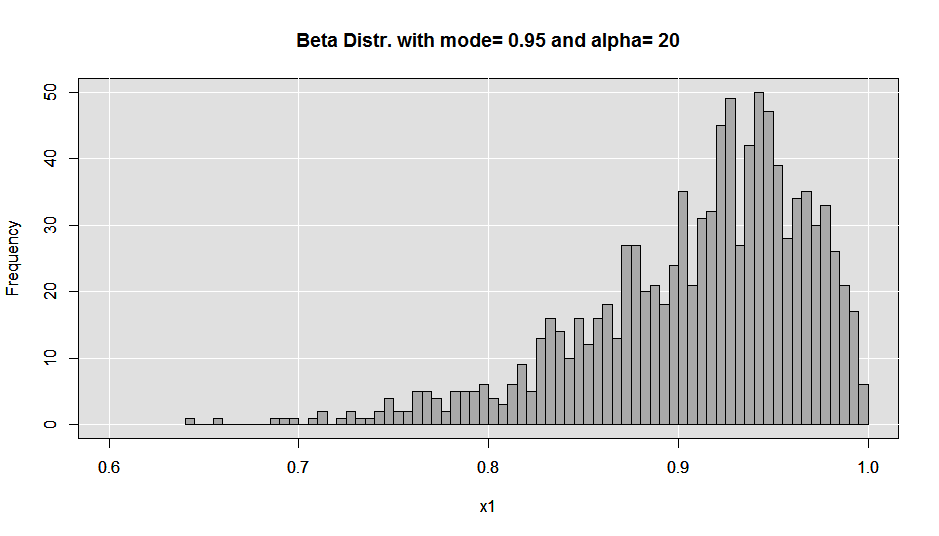
# Now by mode
a2 <- 20
mo1 <- .95
solmode <- function(alpha, mode) (alpha-1-(mode*alpha)+(2*mode))/mode
beta <- solmode(a2, mo1)
x1 <- (rbeta(1000, shape1=a2, shape2=beta)) # sample of n=1000 from the beta dist
head(x1)
x1 <- round(x1,3)
xlimits <- pretty(range(x1))[c(1,length(pretty(range(x1))))]
hist(x1, breaks=100, xlim=xlimits, main="")# let's give it a look
test <- (x1, breaks=100, xlim=xlimits, main="")
u <- par("usr")
rect(u[1], u[3], u[2], u[4], col = "gray88", border = "black")
abline(v = pretty((range(x1))), col='white') ## draw h lines
abline(h = pretty(test$counts), col='white') ## draw h lines
par(new=T)
hist(x1, breaks=100, xlim=xlimits, col='darkgrey', main=paste('Beta Distr. with mode=', mo1, 'and alpha=', a2))# let's give it a look
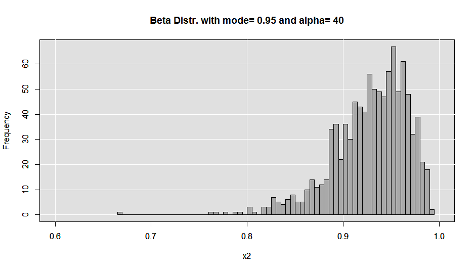
# Now by mode
a2 <- 40
mo1 <- .95
solmode <- function(alpha, mode) (alpha-1-(mode*alpha)+(2*mode))/mode
beta <- solmode(a2, mo1)
x2 <- (rbeta(1000, shape1=a2, shape2=beta)) # sample of n=1000 from the beta dist
head(x2)
x2 <- round(x2,3)
hist(x2, breaks=50, xlim=xlimits, main="")# let's give it a look
test <- hist(x2, breaks=50, xlim=xlimits, main="")
u <- par("usr")
rect(u[1], u[3], u[2], u[4], col = "gray88", border = "black")
abline(v = pretty((range(x1))), col='white') ## draw h lines
abline(h = pretty(test$counts), col='white') ## draw h lines
par(new=T)
hist(x2, breaks=50, xlim=xlimits, col='darkgrey', main=paste('Beta Distr. with mode=', mo1, 'and alpha=', a2))# let's give it a look
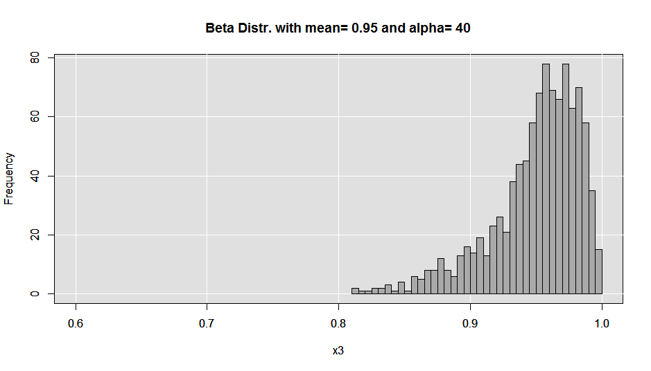
# Now by mean
a3 <- 40
mu1 <- .95
solmean <- function(alpha, mean) (alpha-(mean*alpha))/mean
beta <- solmean(a3, mu1)
x3 <- (rbeta(1000, shape1=a1, shape2=beta)) # sample of n=1000 from the beta dist
head(x3)
mean(x3)
x3 <- round(x3,3)
hist(x3, breaks=50, xlim=xlimits, main="")# let's give it a look
test <- hist(x3, breaks=50, xlim=xlimits, main="")
u <- par("usr")
rect(u[1], u[3], u[2], u[4], col = "gray88", border = "black")
abline(v = pretty((range(x1))), col='white') ## draw h lines
abline(h = pretty(test$counts), col='white') ## draw h lines
par(new=T)
hist(x3, breaks=50, xlim=xlimits, col='darkgrey', main=paste('Beta Distr. with mean=', mu1, 'and alpha=', a3))# let's give it a look
That’s it. I’ve noticed that changing your prespecified alpha does some interesting things to the kurtosis of the resulting beta distribution, but it’s up to you to play around with things until you get a distribution that suits your needs!
One last thing… if you are really into fat-tailed distributions (let’s say your a black swan fan), and you really don’t require a “curvy” form. One great way to sample from a skewed distribution that is realtively easy to specify (in terms of a mode–that is), I’ve found that the triangle package (http://cran.r-project.org/web/packages/triangle/index.html) a nice way to go…. and the code is super easy to run.
 require(triange)
 tri <- round(rtriangle(10000, 0, 1, .85),3)  # just feed it the sample size, min bound, max bound, and mode... and voila!
 hist(tri)
ENJOY!
