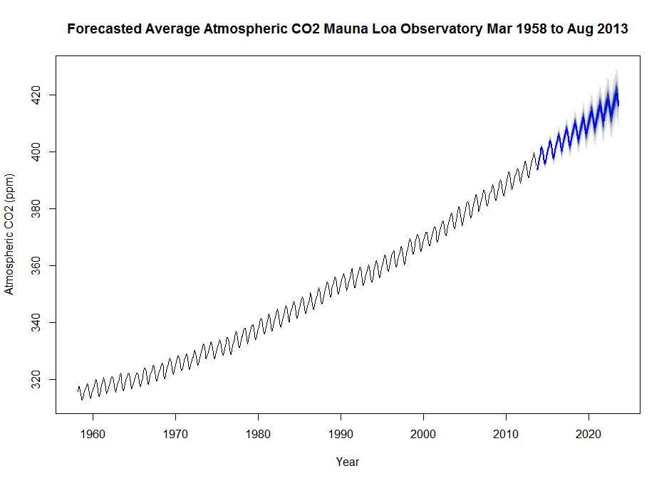
Some time ago, I stumbled upon Rob Hyndman and George Athana­sopou­los’s online text “Forecasting: principles and practice”, and I’ve been really excited to put Rob Hyndman’s forecast package to use, which I did with some client data that I had lying around. Since I could not post the details of that excercise here, I went in search of some publicly available data that I could showcase, and I stumbled upon the Mauna Loa observatory atmospheric CO2 readings. These data describe average atmospheric CO2 readings that go back as far as March of 1958. After decomposing the time series with STL decomposition, I used forecast to forecast what the next 10 years may have in store, given the current trends and pattern of seasonality. There is nothing new or interesting about the trend (check out the trend portion of the decomposition, we’ve all seen these data already reported in one form or another), and initially, while I thought that the pattern of the RATIO of “high-side” remainders to “low-side” remainders appeared to have changed in the early vs. the later years (check out the remainder portion of the decomposition). Where, in the early years, the “high side” remainders were more frequent and of greater relative magnitude then the “low-side” remainders. I did some back-of-the-envelope analysis of the remainders and found that this initial thought doesn’t appear to hold up (code below).

library(forecast)
library(zoo)

file <- "ftp://ftp.cmdl.noaa.gov/ccg/co2/trends/co2_mm_mlo.txt"
xnames <- c("year", "month", "dedcimaldate", "average", "interpolated", "trend_sc", "days_data")

raw_data <- read.table(file, header=FALSE, sep="", skip=72, col.names=xnames)


mintvec <- c( as.numeric((raw_data$year[1])), as.numeric((raw_data$month[1])))
maxtvec <- c( as.numeric((raw_data$year[nrow(raw_data)])), as.numeric((raw_data$month[nrow(raw_data)])))
CO2ts <- ts(raw_data$interpolated, start=(mintvec), end=(maxtvec), frequency=12)


startdate <- as.yearmon(paste(start(CO2ts)[1], start(CO2ts)[2], sep="-"))
enddate <- as.yearmon(paste(end(CO2ts)[1], end(CO2ts)[2], sep="-"))
daterange <- paste(startdate, enddate, sep=" to ")
plot(CO2ts,xlab="Year", ylab= "Atmospheric CO2 (ppm)" ,main=paste("Average Atmospheric CO2 Mauna Loa Observatory", daterange))

fit <- stl(CO2ts, s.window=12, robust=TRUE)

plot(fit, main="Decomposition of Average Atmospheric CO2")

fcast <- forecast(fit, h=120,level=c(50,95), fan=TRUE)
plot(fcast, xlab="Year", ylab= "Atmospheric CO2 (ppm)" ,main=paste("Forecasted Average Atmospheric CO2 Mauna Loa Observatory", daterange))
u <- par("usr")
rect(u[1], u[3], u[2], u[4], col = "gray88", border = "black")
abline(v = pretty(pretty(time(CO2ts))), col='white') ## draw h lines
xrange <- c(range(CO2ts), range(fcast$mean))
xrange <- range(xrange)
abline(h = (pretty(xrange)), col='white') ## draw v lines
par(new=T)
plot(fcast, xlab="Year", ylab= "Atmospheric CO2 (ppm)" ,main=paste("Forecasted Average Atmospheric CO2 Mauna Loa Observatory", daterange))


V1 = seq(from=as.yearmon("Mar 1958"), to=as.yearmon("Aug 2013"), by=1/12)
dfrem <- data.frame( yearmon = V1, remainder = fcast$residuals)
plot(dfrem$remainder, dfrem$V1)
abline(lm(dfrem$remainder~dfrem$yearmon), col='black', lty=3, lwd=2) 
plot(lm(dfrem$remainder~dfrem$yearmon))