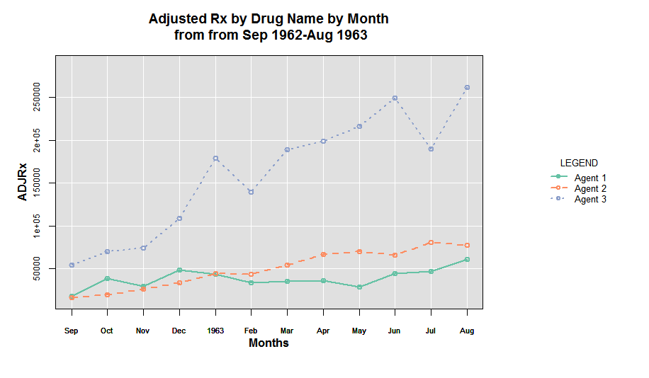
I have waffled back-and-forth from base plotting to ggplot2 back to base plotting for my every day plotting needs. Mainly, this is because when it comes to customization of all aspects of the plot (esp. the legend) I feel more more in command with the base R plotting code. That said, one of the great benefits of ggplot is efficiency and how the package allows users to do quite a lot with very few lines. I certainly still find ggplot2 to be a very handy package!
One of these killer features is the facet option. To achieve something similar with base R takes quite a bit of code to achieve (as far as I can tell), and while I have managed to hackishly create my own base plot work-around, it certainly is far from elegant.

df1 <- structure(list(yearmon = structure(c(1962.66666666667, 1962.75, 
1962.83333333333, 1962.91666666667, 1963, 1963.08333333333, 1963.16666666667, 
1963.25, 1963.33333333333, 1963.41666666667, 1963.5, 1963.58333333333, 
1962.66666666667, 1962.75, 1962.83333333333, 1962.91666666667, 
1963, 1963.08333333333, 1963.16666666667, 1963.25, 1963.33333333333, 
1963.41666666667, 1963.5, 1963.58333333333, 1962.66666666667, 
1962.75, 1962.83333333333, 1962.91666666667, 1963, 1963.08333333333, 
1963.16666666667, 1963.25, 1963.33333333333, 1963.41666666667, 
1963.5, 1963.58333333333), class = "yearmon"), Drug_Name = c("Agent 1", 
"Agent 1", "Agent 1", "Agent 1", "Agent 1", "Agent 1", "Agent 1", 
"Agent 1", "Agent 1", "Agent 1", "Agent 1", "Agent 1", "Agent 2", 
"Agent 2", "Agent 2", "Agent 2", "Agent 2", "Agent 2", "Agent 2", 
"Agent 2", "Agent 2", "Agent 2", "Agent 2", "Agent 2", "Agent 3", 
"Agent 3", "Agent 3", "Agent 3", "Agent 3", "Agent 3", "Agent 3", 
"Agent 3", "Agent 3", "Agent 3", "Agent 3", "Agent 3"), adjrx = c(18143.5783886275, 
38325.3886392513, 28947.4502791512, 48214.462366663, 43333.2885400775, 
33764.6938232197, 35212.886019669, 36189.6070599246, 28200.3430203372, 
43933.5384644003, 46732.6291571359, 60815.5882493688, 15712.9069922491, 
19251.420642945, 25798.4830512904, 33358.078739438, 44149.0834359141, 
43398.7462134831, 54262.7250247334, 66436.6057335244, 69902.3540414917, 
65782.8992544251, 80473.8038710182, 77450.9502630631, 54513.3449101778, 
69888.3308038326, 73786.2648409879, 108656.505665252, 179029.671628446, 
139676.077252012, 188805.180975972, 199308.502689428, 216174.290372019, 
249180.973882092, 189528.429468574, 261748.967406539)), .Names = c("yearmon", 
"Drug_Name", "adjrx"), class = "data.frame", row.names = c(36L, 
39L, 45L, 38L, 41L, 37L, 42L, 34L, 44L, 40L, 35L, 43L, 20L, 17L, 
18L, 15L, 16L, 12L, 14L, 13L, 19L, 21L, 11L, 10L, 33L, 25L, 24L, 
32L, 23L, 22L, 28L, 26L, 30L, 27L, 31L, 29L))

yrange <- paste('from', paste(range(df1$yearmon), collapse="-"))


yval <- 'adjrx'
loopcol <- 'Drug_Name'
xval <- 'yearmon'
ylabtxt <- 'ADJRx'
xlabtxt <- 'Months'
titletxt <- paste(client, ptargetclass, 'Adjusted Rx by Drug Name by Month\n from', yrange)

# ppi <- 300
# png(paste(client, targetclass, 'Drug_Name_adjrx_bymo.png', sep="_"), width=10*ppi, height=6*ppi, res=ppi)
par(mar=c(5.1, 4.1, 4.1, 12.2))
ymax <-  max( df1[c(yval)])+(0.1* max( df1[c(yval)]))
ymin <-  min( df1[c(yval)])-(0.1* min( df1[c(yval)]))
xmax <- max(df1[,c(xval)])
xmin <- min(df1[,c(xval)])
loopvec <- unique(df1[,loopcol])

library(RColorBrewer)
cpal <- brewer.pal(length(loopvec), 'Set2')
plot( df1[,xval], df1[,yval],yaxt='n', xaxt='n', ylab="", xlab="", ylim=c(ymin,ymax))
u <- par("usr")
rect(u[1], u[3], u[2], u[4], col = "gray88", border = "black")
par(new=T)
abline(h = pretty(ymin:ymax), col='white') ##  draw h lines
abline(v = (unique(df1[,xval])), col='white') ##  draw v lines
par(new=T)
for (i in 1:length(loopvec)){
  loopi <- loopvec[i] ##  calls variable to be plotted
  sgi <- df1[ df1[,c(loopcol)] == loopi, ]
  sgi <- sgi[order(sgi[,c(xval)]),]
  plot( sgi[,xval], sgi[, yval], type="o", col=cpal[i], lwd=2, lty=i,yaxt='n', cex.axis=.7, cex.sub=.8, cex.lab=.8, xlab= "", ylab="", ylim=c(ymin,ymax), xlim=c(xmin, xmax)  ,sub=paste('' ), cex.sub=.8)
  if (i < length(loopvec))
    par(new=T)
}
##draw OLS for total

axis(side=2, at= pretty(range(ymin, ymax)), labels=pretty(range(ymin, ymax)), cex.axis=.75, )
mtext(ylabtxt, side=2, line=2, cex.lab=1,las=2,  las=0, font=2)
mtext(xlabtxt, side=1, line=2, cex.lab=1,las=2,  las=0, font=2)
mtext( titletxt, side=3, line=1, font=2, cex=1.2)
legend(xpd=TRUE,'right', inset=c(-0.30,0), legend=loopvec, lwd=rep(2, length(loopvec)), pch=rep(1, length(loopvec)), col=cpal, lty= 1:length(loopvec) ,title="LEGEND", bty='n' , cex=.8)
# dev.off()